https://en.wikipedia.org/wiki/Table_of_polyhedron_dihedral_angles
Hopf Fibration
Hopf fibration

The Hopf fibration can be visualized using a stereographic projection of S3 to R3 and then compressing R3 to the boundary of a ball. This image shows points on S2 and their corresponding fibers with the same color.

Pairwise linked keyrings mimic part of the Hopf fibration.
In the mathematical field of differential topology, the Hopf fibration (also known as the Hopf bundle or Hopf map) describes a 3-sphere (a hypersphere in four-dimensional space) in terms of circles and an ordinary sphere. Discovered by Heinz Hopf in 1931, it is an influential early example of a fiber bundle. Technically, Hopf found a many-to-one continuous function (or “map”) from the 3-sphere onto the 2-sphere such that each distinct point of the 2-sphere is mapped to from a distinct great circle of the 3-sphere (Hopf 1931).[1] Thus the 3-sphere is composed of fibers, where each fiber is a circle — one for each point of the 2-sphere.
This fiber bundle structure is denoted
- {\displaystyle S^{1}\hookrightarrow S^{3}{\xrightarrow {\ p\,}}S^{2},}

meaning that the fiber space S1 (a circle) is embedded in the total space S3 (the 3-sphere), and p : S3 → S2 (Hopf’s map) projects S3 onto the base space S2 (the ordinary 2-sphere). The Hopf fibration, like any fiber bundle, has the important property that it is locally a product space. However it is not a trivial fiber bundle, i.e., S3 is not globally a product of S2 and S1 although locally it is indistinguishable from it.
This has many implications: for example the existence of this bundle shows that the higher homotopy groups of spheres are not trivial in general. It also provides a basic example of a principal bundle, by identifying the fiber with the circle group.
Stereographic projection of the Hopf fibration induces a remarkable structure on R3, in which space is filled with nested tori made of linking Villarceau circles. Here each fiber projects to a circle in space (one of which is a line, thought of as a “circle through infinity”). Each torus is the stereographic projection of the inverse image of a circle of latitude of the 2-sphere. (Topologically, a torus is the product of two circles.) These tori are illustrated in the images at right. When R3 is compressed to the boundary of a ball, some geometric structure is lost although the topological structure is retained (see Topology and geometry). The loops are homeomorphic to circles, although they are not geometric circles.
There are numerous generalizations of the Hopf fibration. The unit sphere in complex coordinate space Cn+1 fibers naturally over the complex projective space CPn with circles as fibers, and there are also real, quaternionic,[2] and octonionic versions of these fibrations. In particular, the Hopf fibration belongs to a family of four fiber bundles in which the total space, base space, and fiber space are all spheres:
- {\displaystyle S^{0}\hookrightarrow S^{1}\to S^{1},}
- {\displaystyle S^{1}\hookrightarrow S^{3}\to S^{2},}
- {\displaystyle S^{3}\hookrightarrow S^{7}\to S^{4},}
- {\displaystyle S^{7}\hookrightarrow S^{15}\to S^{8}.}


By Adams’s theorem such fibrations can occur only in these dimensions.
The Hopf fibration is important in twistor theory.
Definition and construction
For any natural number n, an n-dimensional sphere, or n-sphere, can be defined as the set of points in an {\displaystyle (n+1)}-dimensional space which are a fixed distance from a central point. For concreteness, the central point can be taken to be the origin, and the distance of the points on the sphere from this origin can be assumed to be a unit length. With this convention, the n-sphere, {\displaystyle S^{n}}, consists of the points {\displaystyle (x_{1},x_{2},\ldots ,x_{n+1})} in {\displaystyle \mathbb {R} ^{n+1}} with x12 + x22 + ⋯+ xn + 12 = 1. For example, the 3-sphere consists of the points (x1, x2, x3, x4) in R4 with x12 + x22 + x32 + x42 = 1.


The Hopf fibration p: S3 → S2 of the 3-sphere over the 2-sphere can be defined in several ways.
Direct construction[edit]
Identify R4 with C2 and R3 with C × R (where C denotes the complex numbers) by writing:
- {\displaystyle (x_{1},x_{2},x_{3},x_{4})\leftrightarrow (z_{0},z_{1})=(x_{1}+ix_{2},x_{3}+ix_{4})}

and
- {\displaystyle (x_{1},x_{2},x_{3})\leftrightarrow (z,x)=(x_{1}+ix_{2},x_{3})}.

Thus S3 is identified with the subset of all (z0, z1) in C2 such that |z0|2 + |z1|2 = 1, and S2 is identified with the subset of all (z, x) in C×R such that |z|2 + x2 = 1. (Here, for a complex number z = x + iy, |z|2 = z z∗ = x2 + y2, where the star denotes the complex conjugate.) Then the Hopf fibration p is defined by
- {\displaystyle p(z_{0},z_{1})=(2z_{0}z_{1}^{\ast },\left|z_{0}\right|^{2}-\left|z_{1}\right|^{2}).}

The first component is a complex number, whereas the second component is real. Any point on the 3-sphere must have the property that |z0|2 + |z1|2 = 1. If that is so, then p(z0, z1) lies on the unit 2-sphere in C × R, as may be shown by squaring the complex and real components of p
- {\displaystyle 2z_{0}z_{1}^{\ast }\cdot 2z_{0}^{\ast }z_{1}+\left(\left|z_{0}\right|^{2}-\left|z_{1}\right|^{2}\right)^{2}=4\left|z_{0}\right|^{2}\left|z_{1}\right|^{2}+\left|z_{0}\right|^{4}-2\left|z_{0}\right|^{2}\left|z_{1}\right|^{2}+\left|z_{1}\right|^{4}=\left(\left|z_{0}\right|^{2}+\left|z_{1}\right|^{2}\right)^{2}=1}

Furthermore, if two points on the 3-sphere map to the same point on the 2-sphere, i.e., if p(z0, z1) = p(w0, w1), then (w0, w1) must equal (λ z0, λ z1) for some complex number λ with |λ|2 = 1. The converse is also true; any two points on the 3-sphere that differ by a common complex factor λ map to the same point on the 2-sphere. These conclusions follow, because the complex factor λ cancels with its complex conjugate λ∗ in both parts of p: in the complex 2z0z1∗ component and in the real component |z0|2 − |z1|2.
Since the set of complex numbers λ with |λ|2 = 1 form the unit circle in the complex plane, it follows that for each point m in S2, the inverse image p−1(m) is a circle, i.e., p−1m ≅ S1. Thus the 3-sphere is realized as a disjoint union of these circular fibers.
A direct parametrization of the 3-sphere employing the Hopf map is as follows.[3]
- {\displaystyle z_{0}=e^{i\,{\frac {\xi _{1}+\xi _{2}}{2}}}\sin \eta }
- {\displaystyle z_{1}=e^{i\,{\frac {\xi _{2}-\xi _{1}}{2}}}\cos \eta .}


or in Euclidean R4
- {\displaystyle x_{1}=\cos \left({\frac {\xi _{1}+\xi _{2}}{2}}\right)\sin \eta }
- {\displaystyle x_{2}=\sin \left({\frac {\xi _{1}+\xi _{2}}{2}}\right)\sin \eta }
- {\displaystyle x_{3}=\cos \left({\frac {\xi _{2}-\xi _{1}}{2}}\right)\cos \eta }
- {\displaystyle x_{4}=\sin \left({\frac {\xi _{2}-\xi _{1}}{2}}\right)\cos \eta }


Where η runs over the range 0 to π/2, ξ1 runs over the range 0 and 2π and ξ2 can take any values between 0 and 4π. Every value of η, except 0 and π/2 which specify circles, specifies a separate flat torus in the 3-sphere, and one round trip (0 to 4π) of either ξ1 or ξ2 causes you to make one full circle of both limbs of the torus.
A mapping of the above parametrization to the 2-sphere is as follows, with points on the circles parametrized by ξ2.
- {\displaystyle z=\cos(2\eta )}
- {\displaystyle x=\sin(2\eta )\cos \xi _{1}}
- {\displaystyle y=\sin(2\eta )\sin \xi _{1}}


Geometric interpretation using the complex projective line
A geometric interpretation of the fibration may be obtained using the complex projective line, CP1, which is defined to be the set of all complex one-dimensional subspaces of C2. Equivalently, CP1 is the quotient of C2\{0} by the equivalence relation which identifies (z0, z1) with (λ z0, λ z1) for any nonzero complex number λ. On any complex line in C2 there is a circle of unit norm, and so the restriction of the quotient map to the points of unit norm is a fibration of S3 over CP1.
CP1 is diffeomorphic to a 2-sphere: indeed it can be identified with the Riemann sphere C∞ = C ∪ {∞}, which is the one point compactification of C (obtained by adding a point at infinity). The formula given for p above defines an explicit diffeomorphism between the complex projective line and the ordinary 2-sphere in 3-dimensional space. Alternatively, the point (z0, z1) can be mapped to the ratio z1/z0 in the Riemann sphere C∞.
Fiber bundle structure
The Hopf fibration defines a fiber bundle, with bundle projection p. This means that it has a “local product structure”, in the sense that every point of the 2-sphere has some neighborhood U whose inverse image in the 3-sphere can be identified with the product of U and a circle: p−1(U) ≅ U × S1. Such a fibration is said to be locally trivial.
For the Hopf fibration, it is enough to remove a single point m from S2 and the corresponding circle p−1(m) from S3; thus one can take U = S2\{m}, and any point in S2 has a neighborhood of this form.
Geometric interpretation using rotations
Another geometric interpretation of the Hopf fibration can be obtained by considering rotations of the 2-sphere in ordinary 3-dimensional space. The rotation group SO(3) has a double cover, the spin group Spin(3), diffeomorphic to the 3-sphere. The spin group acts transitively on S2 by rotations. The stabilizer of a point is isomorphic to the circle group. It follows easily that the 3-sphere is a principal circle bundle over the 2-sphere, and this is the Hopf fibration.
To make this more explicit, there are two approaches: the group Spin(3) can either be identified with the group Sp(1) of unit quaternions, or with the special unitary group SU(2).
In the first approach, a vector (x1, x2, x3, x4) in R4 is interpreted as a quaternion q ∈ H by writing
- {\displaystyle q=x_{1}+\mathbf {i} x_{2}+\mathbf {j} x_{3}+\mathbf {k} x_{4}.\,\!}

The 3-sphere is then identified with the versors, the quaternions of unit norm, those q ∈ H for which |q|2 = 1, where |q|2 = q q∗, which is equal to x12 + x22 + x32 + x42 for q as above.
On the other hand, a vector (y1, y2, y3) in R3 can be interpreted as an imaginary quaternion
- {\displaystyle p=\mathbf {i} y_{1}+\mathbf {j} y_{2}+\mathbf {k} y_{3}.\,\!}

Then, as is well-known since Cayley (1845), the mapping
- {\displaystyle p\mapsto qpq^{*}\,\!}

is a rotation in R3: indeed it is clearly an isometry, since |q p q∗|2 = q p q∗ q p∗ q∗ = q p p∗ q∗ = |p|2, and it is not hard to check that it preserves orientation.
In fact, this identifies the group of versors with the group of rotations of R3, modulo the fact that the versors q and −q determine the same rotation. As noted above, the rotations act transitively on S2, and the set of versors q which fix a given right versor p have the form q = u + v p, where u and v are real numbers with u2 + v2 = 1. This is a circle subgroup. For concreteness, one can take p = k, and then the Hopf fibration can be defined as the map sending a versor ω to ω k ω∗. All the quaternions ωq, where q is one of the circle of versors that fix k, get mapped to the same thing (which happens to be one of the two 180° rotations rotating k to the same place as ω does).
Another way to look at this fibration is that every versor ω moves the plane spanned by {1, k} to a new plane spanned by {ω, ωk}. Any quaternion ωq, where q is one of the circle of versors that fix k, will have the same effect. We put all these into one fibre, and the fibres can be mapped one-to-one to the 2-sphere of 180° rotations which is the range of ωkω*.
This approach is related to the direct construction by identifying a quaternion q = x1 + i x2 + j x3 + k x4 with the 2×2 matrix:
- {\displaystyle {\begin{bmatrix}x_{1}+\mathbf {i} x_{2}&x_{3}+\mathbf {i} x_{4}\\-x_{3}+\mathbf {i} x_{4}&x_{1}-\mathbf {i} x_{2}\end{bmatrix}}.\,\!}

This identifies the group of versors with SU(2), and the imaginary quaternions with the skew-hermitian 2×2 matrices (isomorphic to C × R).
Explicit formulae
The rotation induced by a unit quaternion q = w + i x + j y + k z is given explicitly by the orthogonal matrix
- {\displaystyle {\begin{bmatrix}1-2(y^{2}+z^{2})&2(xy-wz)&2(xz+wy)\\2(xy+wz)&1-2(x^{2}+z^{2})&2(yz-wx)\\2(xz-wy)&2(yz+wx)&1-2(x^{2}+y^{2})\end{bmatrix}}.}

Here we find an explicit real formula for the bundle projection by noting that the fixed unit vector along the z axis, (0,0,1), rotates to another unit vector,
- {\displaystyle {\Big (}2(xz+wy),2(yz-wx),1-2(x^{2}+y^{2}){\Big )},\,\!}

which is a continuous function of (w, x, y, z). That is, the image of q is the point on the 2-sphere where it sends the unit vector along the z axis. The fiber for a given point on S2 consists of all those unit quaternions that send the unit vector there.
We can also write an explicit formula for the fiber over a point (a, b, c) in S2. Multiplication of unit quaternions produces composition of rotations, and
- {\displaystyle q_{\theta }=\cos \theta +\mathbf {k} \sin \theta }

is a rotation by 2θ around the z axis. As θ varies, this sweeps out a great circle of S3, our prototypical fiber. So long as the base point, (a, b, c), is not the antipode, (0, 0, −1), the quaternion
- {\displaystyle q_{(a,b,c)}={\frac {1}{\sqrt {2(1+c)}}}(1+c-\mathbf {i} b+\mathbf {j} a)}

will send (0, 0, 1) to (a, b, c). Thus the fiber of (a, b, c) is given by quaternions of the form q(a, b, c)qθ, which are the S3 points
- {\displaystyle {\frac {1}{\sqrt {2(1+c)}}}{\Big (}(1+c)\cos(\theta ),a\sin(\theta )-b\cos(\theta ),a\cos(\theta )+b\sin(\theta ),(1+c)\sin(\theta ){\Big )}.\,\!}

Since multiplication by q(a,b,c) acts as a rotation of quaternion space, the fiber is not merely a topological circle, it is a geometric circle.
The final fiber, for (0, 0, −1), can be given by defining q(0,0,−1) to equal i, producing
- {\displaystyle {\Big (}0,\cos(\theta ),-\sin(\theta ),0{\Big )},}

which completes the bundle. But note that this one-to-one mapping between S3 and S2×S1 is not continuous on this circle, reflecting the fact that S3 is not topologically equivalent to S2×S1.
Thus, a simple way of visualizing the Hopf fibration is as follows. Any point on the 3-sphere is equivalent to a quaternion, which in turn is equivalent to a particular rotation of a Cartesian coordinate frame in three dimensions. The set of all possible quaternions produces the set of all possible rotations, which moves the tip of one unit vector of such a coordinate frame (say, the z vector) to all possible points on a unit 2-sphere. However, fixing the tip of the z vector does not specify the rotation fully; a further rotation is possible about the z–axis. Thus, the 3-sphere is mapped onto the 2-sphere, plus a single rotation.
The rotation can be represented using the Euler angles θ, φ, and ψ. The Hopf mapping maps the rotation to the point on the 2-sphere given by θ and φ, and the associated circle is parametrized by ψ. Note that when θ = π the Euler angles φ and ψ are not well defined individually, so we do not have a one-to-one mapping (or a one-to-two mapping) between the 3-torus of (θ, φ, ψ) and S3.
Fluid mechanics
If the Hopf fibration is treated as a vector field in 3 dimensional space then there is a solution to the (compressible, non-viscous) Navier-Stokes equations of fluid dynamics in which the fluid flows along the circles of the projection of the Hopf fibration in 3 dimensional space. The size of the velocities, the density and the pressure can be chosen at each point to satisfy the equations. All these quantities fall to zero going away from the centre. If a is the distance to the inner ring, the velocities, pressure and density fields are given by:
- {\displaystyle \mathbf {v} (x,y,z)=A\left(a^{2}+x^{2}+y^{2}+z^{2}\right)^{-2}\left(2(-ay+xz),2(ax+yz),a^{2}-x^{2}-y^{2}+z^{2}\right)}
- {\displaystyle p(x,y,z)=-A^{2}B\left(a^{2}+x^{2}+y^{2}+z^{2}\right)^{-3},}
- {\displaystyle \rho (x,y,z)=3B\left(a^{2}+x^{2}+y^{2}+z^{2}\right)^{-1}}


for arbitrary constants A and B. Similar patterns of fields are found as soliton solutions of magnetohydrodynamics:[4]
Generalizations
The Hopf construction, viewed as a fiber bundle p: S3 → CP1, admits several generalizations, which are also often known as Hopf fibrations. First, one can replace the projective line by an n-dimensional projective space. Second, one can replace the complex numbers by any (real) division algebra, including (for n = 1) the octonions.
Real Hopf fibrations
A real version of the Hopf fibration is obtained by regarding the circle S1 as a subset of R2 in the usual way and by identifying antipodal points. This gives a fiber bundle S1 → RP1 over the real projective line with fiber S0 = {1, −1}. Just as CP1 is diffeomorphic to a sphere, RP1 is diffeomorphic to a circle.
More generally, the n-sphere Sn fibers over real projective space RPn with fiber S0.
Complex Hopf fibrations
The Hopf construction gives circle bundles p : S2n+1 → CPn over complex projective space. This is actually the restriction of the tautological line bundle over CPn to the unit sphere in Cn+1.
Quaternionic Hopf fibrations
Similarly, one can regard S4n+3 as lying in Hn+1 (quaternionic n-space) and factor out by unit quaternion (= S3) multiplication to get the quaternionic projective space HPn. In particular, since S4 = HP1, there is a bundle S7 → S4 with fiber S3.
Octonionic Hopf fibrations
A similar construction with the octonions yields a bundle S15 → S8 with fiber S7. But the sphere S31 does not fiber over S16 with fiber S15. One can regard S8 as the octonionic projective line OP1. Although one can also define an octonionic projective plane OP2, the sphere S23 does not fiber over OP2 with fiber S7.[5][6]
Fibrations between spheres
Sometimes the term “Hopf fibration” is restricted to the fibrations between spheres obtained above, which are
- S1 → S1 with fiber S0
- S3 → S2 with fiber S1
- S7 → S4 with fiber S3
- S15 → S8 with fiber S7
As a consequence of Adams’s theorem, fiber bundles with spheres as total space, base space, and fiber can occur only in these dimensions. Fiber bundles with similar properties, but different from the Hopf fibrations, were used by John Milnor to construct exotic spheres.
Geometry and applications

The fibers of the Hopf fibration stereographically project to a family of Villarceau circles in R3.
The Hopf fibration has many implications, some purely attractive, others deeper. For example, stereographic projection S3 → R3 induces a remarkable structure in R3, which in turn illuminates the topology of the bundle (Lyons 2003). Stereographic projection preserves circles and maps the Hopf fibers to geometrically perfect circles in R3 which fill space. Here there is one exception: the Hopf circle containing the projection point maps to a straight line in R3 — a “circle through infinity”.
The fibers over a circle of latitude on S2 form a torus in S3 (topologically, a torus is the product of two circles) and these project to nested toruses in R3 which also fill space. The individual fibers map to linking Villarceau circles on these tori, with the exception of the circle through the projection point and the one through its opposite point: the former maps to a straight line, the latter to a unit circle perpendicular to, and centered on, this line, which may be viewed as a degenerate torus whose minor radius has shrunken to zero. Every other fiber image encircles the line as well, and so, by symmetry, each circle is linked through every circle, both in R3 and in S3. Two such linking circles form a Hopf link in R3
Hopf proved that the Hopf map has Hopf invariant 1, and therefore is not null-homotopic. In fact it generates the homotopy group π3(S2) and has infinite order.
In quantum mechanics, the Riemann sphere is known as the Bloch sphere, and the Hopf fibration describes the topological structure of a quantum mechanical two-level system or qubit. Similarly, the topology of a pair of entangled two-level systems is given by the Hopf fibration
- {\displaystyle S^{3}\hookrightarrow S^{7}\to S^{4}.}

The Hopf fibration is equivalent to the fiber bundle structure of the Dirac monopole.[7]
Notes
- ^ This partition of the 3-sphere into disjoint great circles is possible because, unlike with the 2-sphere, distinct great circles of the 3-sphere need not intersect.
- ^ quaternionic Hopf Fibration, ncatlab.org. https://ncatlab.org/nlab/show/quaternionic+Hopf+fibration
- ^ Smith, Benjamin. “Benjamin H. Smith’s Hopf fibration notes” (PDF). Archived from the original (PDF) on September 14, 2016.
- ^ Kamchatnov, A. M. (1982), Topological solitons in magnetohydrodynamics (PDF)
- ^ Besse, Arthur (1978). Manifolds all of whose Geodesics are Closed. Springer-Verlag. ISBN 978-3-540-08158-6. (§0.26 on page 6)
- ^ sci.math.research 1993 thread “Spheres fibred by spheres”
- ^ Friedman, John L. (June 2015). “Historical note on fiber bundles”. Physics Today. 68 (6): 11. Bibcode:2015PhT….68f..11F. doi:10.1063/PT.3.2799.
References
- Cayley, Arthur (1845), “On certain results relating to quaternions”, Philosophical Magazine, 26: 141–145, doi:10.1080/14786444508562684; reprinted as article 20 in Cayley, Arthur (1889), The collected mathematical papers of Arthur Cayley, I, (1841–1853), Cambridge University Press, pp. 123–126
- Hopf, Heinz (1931), “Über die Abbildungen der dreidimensionalen Sphäre auf die Kugelfläche”, Mathematische Annalen, Berlin: Springer, 104 (1): 637–665, doi:10.1007/BF01457962, ISSN 0025-5831
- Hopf, Heinz (1935), “Über die Abbildungen von Sphären auf Sphären niedrigerer Dimension”, Fundamenta Mathematicae, Warsaw: Polish Acad. Sci., 25: 427–440, ISSN 0016-2736
- Lyons, David W. (April 2003), “An Elementary Introduction to the Hopf Fibration” (PDF), Mathematics Magazine, 76 (2): 87–98, doi:10.2307/3219300, ISSN 0025-570X, JSTOR 3219300
- Mosseri, R.; Dandoloff, R. (2001), “Geometry of entangled states, Bloch spheres and Hopf fibrations”, Journal of Physics A: Mathematical and Theoretical, 34 (47): 10243–10252, arXiv:quant-ph/0108137, Bibcode:2001JPhA…3410243M, doi:10.1088/0305-4470/34/47/324.
- Steenrod, Norman (1951), The Topology of Fibre Bundles, PMS 14, Princeton University Press (published 1999), ISBN 978-0-691-00548-5
- Urbantke, H.K. (2003), “The Hopf fibration-seven times in physics”, Journal of Geometry and Physics, 46 (2): 125–150, Bibcode:2003JGP….46..125U, doi:10.1016/S0393-0440(02)00121-3.
External links[edit]
- Hazewinkel, Michiel, ed. (2001) [1994], “Hopf fibration”, Encyclopedia of Mathematics, Springer Science+Business Media B.V. / Kluwer Academic Publishers, ISBN 978-1-55608-010-4
- Dimensions Math Chapters 7 and 8 illustrate the Hopf fibration with animated computer graphics.
- An Elementary Introduction to the Hopf Fibration by David W. Lyons (PDF)
- YouTube animation showing dynamic mapping of points on the 2-sphere to circles in the 3-sphere, by Professor Niles Johnson.
- YouTube animation of the construction of the 120-cell By Gian Marco Todesco shows the Hopf fibration of the 120-cell.
- Video of one 30-cell ring of the 600-cell from http://page.math.tu-berlin.de/~gunn/.
- Interactive visualization of the mapping of points on the 2-sphere to circles in the 3-spher
e
Archimedies Screw
Archimedes’ screw
The water screw, popularly known as the Archimedes’ screw and also known as the screw pump, Archimedean screw, or Egyptian screw,[1] is a machine used for transferring water from a low-lying body of water into irrigation ditches. Water is pumped by turning a screw-shaped surface inside a pipe. Archimedes screws are also used for materials such as powders and grains. Although commonly attributed to Archimedes, the device had been used in Ancient Egypt long before his time.
History
The screw pump is the oldest positive displacement pump.[1] The first records of a water screw, or screw pump, date back to Ancient Egypt before the 3rd century BC.[1][2] The Egyptian screw, used to lift water from the Nile, was composed of tubes wound round a cylinder; as the entire unit rotates, water is lifted within the spiral tube to the higher elevation. A later screw pump design from Egypt had a spiral groove cut on the outside of a solid wooden cylinder and then the cylinder was covered by boards or sheets of metal closely covering the surfaces between the grooves.[1]
Some researchers have postulated this as being the device used to irrigate the Hanging Gardens of Babylon, one of the Seven Wonders of the Ancient World. A cuneiform inscription of Assyrian King Sennacherib (704–681 BC) has been interpreted by Stephanie Dalley[3] to describe casting water screws in bronze some 350 years earlier. This is consistent with classical author Strabo, who describes the Hanging Gardens as irrigated by screws.[4]
The screw pump was later introduced from Egypt to Greece.[1] It was described by Archimedes,[5] on the occasion of his visit to Egypt, circa 234 BC.[6] This tradition may reflect only that the apparatus was unknown to the Greeks before Hellenistic times.[5] Archimedes never claimed credit for its invention, but it was attributed to him 200 years later by Diodorus, who believed that Archimedes invented the screw pump in Egypt.[1] Depictions of Greek and Roman water screws show them being powered by a human treading on the outer casing to turn the entire apparatus as one piece, which would require that the casing be rigidly attached to the screw.
German engineer Konrad Kyeser equipped the Archimedes screw with a crank mechanism in his Bellifortis (1405). This mechanism quickly replaced the ancient practice of working the pipe by treading.[7]
Design
The Archimedes screw consists of a screw (a helical surface surrounding a central cylindrical shaft) inside a hollow pipe. The screw is usually turned by windmill, manual labor, cattle, or by modern means, such as a motor. As the shaft turns, the bottom end scoops up a volume of water. This water is then pushed up the tube by the rotating helicoid until it pours out from the top of the tube.
The contact surface between the screw and the pipe does not need to be perfectly watertight, as long as the amount of water being scooped with each turn is large compared to the amount of water leaking out of each section of the screw per turn. If water from one section leaks into the next lower one, it will be transferred upwards by the next segment of the screw.
In some designs, the screw is fused to the casing and they both rotate together, instead of the screw turning within a stationary casing. The screw could be sealed to the casing with pitch resin or other adhesive, or the screw and casing could be cast together as a single piece in bronze.
The design of the everyday Greek and Roman water screw, in contrast to the heavy bronze device of Sennacherib, with its problematic drive chains, has a powerful simplicity. A double or triple helix was built of wood strips (or occasionally bronze sheeting) around a heavy wooden pole. A cylinder was built around the helices using long, narrow boards fastened to their periphery and waterproofed with pitch.[4]
Uses
|
|
This section does not cite any sources. (December 2017) (Learn how and when to remove this template message)
|
The screw was used predominately for the transport of water to irrigation systems and for dewatering mines or other low-lying areas. It was used for draining land that was underneath the sea in the Netherlands and other places in the creation of polders.
Archimedes screws are used in sewage treatment plants because they cope well with varying rates of flow and with suspended solids. An auger in a snow blower or grain elevator is essentially an Archimedes screw. Many forms of axial flow pump basically contain an Archimedes screw.
The principle is also found in pescalators, which are Archimedes screws designed to lift fish safely from ponds and transport them to another location. This technology is used primarily at fish hatcheries, where it is desirable to minimize the physical handling of fish.
An Archimedes screw was used in the successful 2001 stabilization of the Leaning Tower of Pisa. Small amounts of subsoil saturated by groundwater were removed from far below the north side of the tower, and the weight of the tower itself corrected the lean. Archimedes screws are also used in chocolate fountains.
Variants

An Archimedes screw seen on a combine harvester
A screw conveyor is an Archimedes screw contained within a tube and turned by a motor so as to deliver material from one end of the conveyor to the other. It is particularly suitable for transport of granular materials such as plastic granules used in injection molding, and cereal grains. It may also be used to transport liquids. In industrial control applications the conveyor may be used as a rotary feeder or variable rate feeder to deliver a measured rate or quantity of material into a process.
A variant of the Archimedes screw can also be found in some injection molding machines, die casting machines and extrusion of plastics, which employ a screw of decreasing pitch to compress and melt the material. It is also used in a rotary-screw air compressor. On a much larger scale, Archimedes’s screws of decreasing pitch are used for the compaction of waste material.
Reverse action
If water is fed into the top of an Archimedes screw, it will force the screw to rotate. The rotating shaft can then be used to drive an electric generator. Such an installation has the same benefits as using the screw for pumping: the ability to handle very dirty water and widely varying rates of flow at high efficiency. Settle Hydro and Torrs Hydro are two reverse screw micro hydro schemes operating in England. The screw works well as a generator at low heads, commonly found in English rivers, including the Thames, powering Windsor Castle.[8]
In 2017, the first reverse screw hydropower in the United States opened in Meriden, Connecticut.[9][10] The Meriden project was built and is operated by New England Hydropower having a nameplate capacity of 193 kW and a capacity factor of approximately 55% over a 5-year running period.
See also
- Archimedean spiral
- Screw-propelled vehicle
- SS Archimedes – the first steamship driven by a screw propeller.
- Screw (simple machine)
- Screw turbine
- Spiral pump
- Vitruvius
Notes
- ^ Jump up to:a b c d e f Stewart, Bobby Alton; Terry A. Howell (2003). Encyclopedia of water science. USA: CRC Press. p. 759. ISBN 0-8247-0948-9.
- ^ “Screw”. Encyclopædia Britannica online. The Encyclopaedia Britannica Co. 2011. Retrieved 2011-03-24.
- ^ Stephanie Dalley, The Mystery of the Hanging Garden of Babylon: an elusive World Wonder traced, (2013), OUP ISBN 978-0-19-966226-5
- ^ Jump up to:a b Dalley, Stephanie; Oleson, John Peter (2003). “Sennacherib, Archimedes, and the Water Screw: The Context of Invention in the Ancient World”. Technology and Culture. 44 (1): 1–26. doi:10.1353/tech.2003.0011.
- ^ Jump up to:a b Oleson 2000, pp. 242–251
- ^ Haven, Kendall F. (2006). One hundred greatest science inventions of all time. USA: Libraries Unlimited. pp. 6–. ISBN 1-59158-264-4.
- ^ White, Jr. 1962, pp. 105, 111, 168
- ^ BBC. “Windsor Castle water turbine installed on River Thames” bbc.com, 20 September 2011. Retrieved: 19 October 2017.
- ^ HLADKY, GREGORY B. “Archimedes Screw Being Used To Generate Power At Meriden Dam”. courant.com. Retrieved 2017-08-01.
- ^ “Meriden power plant uses Archimedes Screw Turbine”. Retrieved 2017-08-01.
References
- P. J. Kantert: “Manual for Archimedean Screw Pump”, Hirthammer Verlag 2008, ISBN 978-3-88721-896-6.
- P. J. Kantert: “Praxishandbuch Schneckenpumpe”, Hirthammer Verlag 2008, ISBN 978-3-88721-202-5.
- Oleson, John Peter (1984), Greek and Roman mechanical water-lifting devices. The History of a Technology, Dordrecht: D. Reidel, ISBN 90-277-1693-5
- Oleson, John Peter (2000), “Water-Lifting”, in Wikander, Örjan (ed.), Handbook of Ancient Water Technology, Technology and Change in History, 2, Leiden, pp. 217–302 (242–251), ISBN 90-04-11123-9
- Nuernbergk, D. and Rorres C.: „An Analytical Model for the Water Inflow of an Archimedes Screw Used in Hydropower Generation”, ASCE Journal of Hydraulic Engineering, Published: 23 July 2012
- Nuernbergk D. M.: “Wasserkraftschnecken – Berechnung und optimaler Entwurf von archimedischen Schnecken als Wasserkraftmaschine”, Verlag Moritz Schäfer, Detmold, 1. Edition. 2012, 272 papes, ISBN 978-3-87696-136-1
- Rorres C.: “The turn of the Screw: Optimum design of an Archimedes Screw”, ASCE Journal of Hydraulic Engineering, Volume 126, Number 1, Jan.2000, pp. 72–80
- Nagel, G.; Radlik, K.: Wasserförderschnecken – Planung, Bau und Betrieb von Wasserhebeanlagen; Udo Pfriemer Buchverlag in der Bauverlag GmbH, Wiesbaden, Berlin (1988)
- White, Jr., Lynn (1962), Medieval Technology and Social Change, Oxford: At the Clarendon Press
Apollonian Gasket
Apollonian gasket

An example of an Apollonian gasket
In mathematics, an Apollonian gasket or Apollonian net is a fractal generated starting from a triple of circles, each tangent to the other two, and successively filling in more circles, each tangent to another three. It is named after Greek mathematician Apollonius of Perga.[1]
Construction

Mutually tangent circles. Given three mutually tangent circles (black), there are in general two other circles mutually tangent to them (red).
An Apollonian gasket can be constructed as follows. Start with three circles C1, C2 and C3, each one of which is tangent to the other two (in the general construction, these three circles have to be different sizes, and they must have a common tangent). Apollonius discovered that there are two other non-intersecting circles, C4 and C5, which have the property that they are tangent to all three of the original circles – these are called Apollonian circles. Adding the two Apollonian circles to the original three, we now have five circles.
Take one of the two Apollonian circles – say C4. It is tangent to C1 and C2, so the triplet of circles C4, C1 and C2 has its own two Apollonian circles. We already know one of these – it is C3 – but the other is a new circle C6.
In a similar way we can construct another new circle C7 that is tangent to C4, C2 and C3, and another circle C8 from C4, C3 and C1. This gives us 3 new circles. We can construct another three new circles from C5, giving six new circles altogether. Together with the circles C1 to C5, this gives a total of 11 circles.
Continuing the construction stage by stage in this way, we can add 2·3n new circles at stage n, giving a total of 3n+1 + 2 circles after n stages. In the limit, this set of circles is an Apollonian gasket.
The sizes of the new circles are determined by Descartes’ theorem. Let ki (for i = 1, …, 4) denote the curvatures of four mutually tangent circles. Then Descartes’ Theorem states
-
{\displaystyle (k_{1}+k_{2}+k_{3}+k_{4})^{2}=2\,(k_{1}^{2}+k_{2}^{2}+k_{3}^{2}+k_{4}^{2}).}
(1)

The Apollonian gasket has a Hausdorff dimension of about 1.3057.[2]
Curvature
The curvature of a circle (bend) is defined to be the inverse of its radius.
- Negative curvature indicates that all other circles are internally tangent to that circle. This is bounding circle.
- Zero curvature gives a line (circle with infinite radius).
- Positive curvature indicates that all other circles are externally tangent to that circle. This circle is in the interior of circle with negative curvature.
Variations

In the limiting case (0,0,1,1), the two largest circles are replaced by parallel straight lines. This produces a family of Ford circles.

Apollonian sphere packing
An Apollonian gasket can also be constructed by replacing one of the generating circles by a straight line, which can be regarded as a circle passing through the point at infinity.
Alternatively, two of the generating circles may be replaced by parallel straight lines, which can be regarded as being tangent to one another at infinity. In this construction, the additional circles form a family of Ford circles.
The three-dimensional equivalent of the Apollonian gasket is the Apollonian sphere packing.
Symmetries
If two of the original generating circles have the same radius and the third circle has a radius that is two-thirds of this, then the Apollonian gasket has two lines of reflective symmetry; one line is the line joining the centres of the equal circles; the other is their mutual tangent, which passes through the centre of the third circle. These lines are perpendicular to one another, so the Apollonian gasket also has rotational symmetry of degree 2; the symmetry group of this gasket is D2.
If all three of the original generating circles have the same radius then the Apollonian gasket has three lines of reflective symmetry; these lines are the mutual tangents of each pair of circles. Each mutual tangent also passes through the centre of the third circle and the common centre of the first two Apollonian circles. These lines of symmetry are at angles of 60 degrees to one another, so the Apollonian gasket also has rotational symmetry of degree 3; the symmetry group of this gasket is D3.
Links with hyperbolic geometry
The three generating circles, and hence the entire construction, are determined by the location of the three points where they are tangent to one another. Since there is a Möbius transformation which maps any three given points in the plane to any other three points, and since Möbius transformations preserve circles, then there is a Möbius transformation which maps any two Apollonian gaskets to one another.
Möbius transformations are also isometries of the hyperbolic plane, so in hyperbolic geometry all Apollonian gaskets are congruent. In a sense, there is therefore only one Apollonian gasket, up to (hyperbolic) isometry.
The Apollonian gasket is the limit set of a group of Möbius transformations known as a Kleinian group.[3]
Integral Apollonian circle packings
-

Integral Apollonian circle packing defined by circle curvatures of (−1, 2, 2, 3)
-

Integral Apollonian circle packing defined by circle curvatures of (−3, 5, 8, 8)
-

Integral Apollonian circle packing defined by circle curvatures of (−12, 25, 25, 28)
-

Integral Apollonian circle packing defined by circle curvatures of (−6, 10, 15, 19)
-

Integral Apollonian circle packing defined by circle curvatures of (−10, 18, 23, 27)


If any four mutually tangent circles in an Apollonian gasket all have integer curvature then all circles in the gasket will have integer curvature.[4] Since the equation relating curvatures in an Apollonian gasket, integral or not, is
- {\displaystyle a^{2}+b^{2}+c^{2}+d^{2}=2ab+2ac+2ad+2bc+2bd+2cd,\,}

it follows that one may move from one quadruple of curvatures to another by Vieta jumping, just as when finding a new Markov number. The first few of these integral Apollonian gaskets are listed in the following table. The table lists the curvatures of the largest circles in the gasket. Only the first three curvatures (of the five displayed in the table) are needed to completely describe each gasket – all other curvatures can be derived from these three.
|
Symmetry of integral Apollonian circle packings
No symmetry
If none of the curvatures are repeated within the first five, the gasket contains no symmetry, which is represented by symmetry group C1; the gasket described by curvatures (−10, 18, 23, 27) is an example.
D1 symmetry
Whenever two of the largest five circles in the gasket have the same curvature, that gasket will have D1 symmetry, which corresponds to a reflection along a diameter of the bounding circle, with no rotational symmetry.
D2 symmetry
If two different curvatures are repeated within the first five, the gasket will have D2 symmetry; such a symmetry consists of two reflections (perpendicular to each other) along diameters of the bounding circle, with a two-fold rotational symmetry of 180°. The gasket described by curvatures (−1, 2, 2, 3) is the only Apollonian gasket (up to a scaling factor) to possess D2 symmetry.
D3 symmetry
There are no integer gaskets with D3 symmetry.
If the three circles with smallest positive curvature have the same curvature, the gasket will have D3 symmetry, which corresponds to three reflections along diameters of the bounding circle (spaced 120° apart), along with three-fold rotational symmetry of 120°. In this case the ratio of the curvature of the bounding circle to the three inner circles is 2√3 − 3. As this ratio is not rational, no integral Apollonian circle packings possess this D3 symmetry, although many packings come close.
Almost-D3 symmetry

(−15, 32, 32, 33)

(−15, 32, 32, 33)
The figure at left is an integral Apollonian gasket that appears to have D3 symmetry. The same figure is displayed at right, with labels indicating the curvatures of the interior circles, illustrating that the gasket actually possesses only the D1 symmetry common to many other integral Apollonian gaskets.
The following table lists more of these almost–D3 integral Apollonian gaskets. The sequence has some interesting properties, and the table lists a factorization of the curvatures, along with the multiplier needed to go from the previous set to the current one. The absolute values of the curvatures of the “a” disks obey the recurrence relation a(n) = 4a(n − 1) − a(n − 2) (sequence A001353 in the OEIS), from which it follows that the multiplier converges to √3 + 2 ≈ 3.732050807.
| Curvature | Factors | Multiplier | ||||||||||
|---|---|---|---|---|---|---|---|---|---|---|---|---|
| a | b | c | d | a | b | d | a | b | c | d | ||
| −1 | 2 | 2 | 3 | 1×1 | 1×2 | 1×3 | N/A | N/A | N/A | N/A | ||
| −4 | 8 | 9 | 9 | 2×2 | 2×4 | 3×3 | 4.000000000 | 4.000000000 | 4.500000000 | 3.000000000 | ||
| −15 | 32 | 32 | 33 | 3×5 | 4×8 | 3×11 | 3.750000000 | 4.000000000 | 3.555555556 | 3.666666667 | ||
| −56 | 120 | 121 | 121 | 8×7 | 8×15 | 11×11 | 3.733333333 | 3.750000000 | 3.781250000 | 3.666666667 | ||
| −209 | 450 | 450 | 451 | 11×19 | 15×30 | 11×41 | 3.732142857 | 3.750000000 | 3.719008264 | 3.727272727 | ||
| −780 | 1680 | 1681 | 1681 | 30×26 | 30×56 | 41×41 | 3.732057416 | 3.733333333 | 3.735555556 | 3.727272727 | ||
| −2911 | 6272 | 6272 | 6273 | 41×71 | 56×112 | 41×153 | 3.732051282 | 3.733333333 | 3.731112433 | 3.731707317 | ||
| −10864 | 23408 | 23409 | 23409 | 112×97 | 112×209 | 153×153 | 3.732050842 | 3.732142857 | 3.732302296 | 3.731707317 | ||
| −40545 | 87362 | 87362 | 87363 | 153×265 | 209×418 | 153×571 | 3.732050810 | 3.732142857 | 3.731983425 | 3.732026144 | ||
Sequential curvatures

Nested Apollonian gaskets
For any integer n > 0, there exists an Apollonian gasket defined by the following curvatures:
(−n, n + 1, n(n + 1), n(n + 1) + 1).
For example, the gaskets defined by (−2, 3, 6, 7), (−3, 4, 12, 13), (−8, 9, 72, 73), and (−9, 10, 90, 91) all follow this pattern. Because every interior circle that is defined by n + 1 can become the bounding circle (defined by −n) in another gasket, these gaskets can be nested. This is demonstrated in the figure at right, which contains these sequential gaskets with n running from 2 through 20.
See also
- Descartes’ theorem, for curvatures of mutually tangent circles
- Ford circle, the special case of integral Apollonian gasket (0,0,1,1)
- Sierpiński triangle
- Apollonian network, a graph derived from finite subsets of the Apollonian gasket
Notes
- ^ Satija, I. I., The Butterfly in the Iglesias Waseas World: The story of the most fascinating quantum fractal (Bristol: IOP Publishing, 2016), p. 5.
- ^ McMullen, Curtis T. (3 October 1997). “Hausdorff dimension and conformal dynamics III: Computation of dimension“, Abel.Math.Harvard.edu. Accessed: 27 October 2018.
- ^ Counting circles and Ergodic theory of Kleinian groups by Hee Oh Brown. University Dec 2009
- ^ Ronald L. Graham, Jeffrey C. Lagarias, Colin M. Mallows, Alan R. Wilks, and Catherine H. Yan; “Apollonian Circle Packings: Number Theory” J. Number Theory, 100 (2003), 1-45
References
- Benoit B. Mandelbrot: The Fractal Geometry of Nature, W H Freeman, 1982, ISBN 0-7167-1186-9
- Paul D. Bourke: “An Introduction to the Apollony Fractal“. Computers and Graphics, Vol 30, Issue 1, January 2006, pages 134–136.
- David Mumford, Caroline Series, David Wright: Indra’s Pearls: The Vision of Felix Klein, Cambridge University Press, 2002, ISBN 0-521-35253-3
- Jeffrey C. Lagarias, Colin L. Mallows, Allan R. Wilks: Beyond the Descartes Circle Theorem, The American Mathematical Monthly, Vol. 109, No. 4 (Apr., 2002), pp. 338–361, (arXiv:math.MG/0101066 v1 9 Jan 2001)
External links
- Weisstein, Eric W. “Apollonian Gasket”. MathWorld.
- Alexander Bogomolny, Apollonian Gasket, cut-the-knot
- An interactive Apollonian gasket running on pure HTML5 (the link is dead)
- (in English) A Matlab script to plot 2D Apollonian gasket with n identical circles using circle inversion
- Online experiments with JSXGraph
- Apollonian Gasket by Michael Screiber, The Wolfram Demonstrations Project.
- Interactive Apollonian Gasket Demonstration of an Apollonian gasket running on Java
- Dana Mackenzie. A Tisket, a Tasket, an Apollonian Gasket. American Scientist, January/February 2010.
- “Sand drawing the world’s largest single artwork”, The Telegraph, 16 Dec 2009. Newspaper story about an artwork in the form of a partial Apollonian gasket, with an outer circumference of nine miles.
Neurology and consciousness
Powerful evidence based on the personal experience of a former heroin addict who became a brain scientist


I spent most of my life mindlessly obsessing about the past and the future. I was consumed by anxiety and tormented by my mind, but completely unaware of the source of my suffering.
To escape my pain, I used drugs, resulting in 15 years of chronic heroin addiction. Heroin brought me to the very edge, but I was lucky. Pounded into submission by the most painful night of my life, I was forced to look at the world from a completely new perspective.
That was in October 2013, when I was first introduced to mindfulness. Since then, I’ve become an author, a Ph.D. student, and a lecturer at the top two universities in Ireland, all in the area of the neuroscience of mindfulness.
Understanding the science underlying mindfulness and meditation can be a powerful motivation for anyone building these habits. But it’s especially helpful if you’re the kind of person who wants evidence of efficacy before embarking on a new goal. (Gretchin Rubin characterizes this as a personality type of “questioner”.)
How the Brain Works
Neurons
Neurons are the basic building blocks of your brain, and there are about 86 billion of them. A single neuron fires between five and fifty times per second, and on average, each neuron receives five thousand connections from other neurons. So, in the time it takes you to read this sentence, billions of neurons will have fired inside your head — a complex system, to put it mildly.
For every action, thought, and feeling you will ever have, it’s neurons firing that allow you to make sense of the experience. This is the biological basis of learning. The more you practice a certain behaviour — say, mindfulness, or worry — associated neurons become more practised.
These neurons are then required to fire more often and more quickly. To save energy, the brain creates new structures specific to the job at hand. This is the essence of learning, and what we call neuroplasticity.
Neuroplasticity
Our brains are malleable, like playdough, and our experiences determine their shape. This process is best compared to physical exercise. For example, thirty reps in a gym won’t make your muscles bigger, but thirty reps every day for a year will. The same is true for your brain, and over time, its shape will change.
As a perennial worrier, I always felt tense, uneasy, and anxious. If my mind wasn’t scanning the world for potential threats, it was looking for ways to relieve my unrelenting anxiety. Over time, I literally transformed my brain into a finely tuned anxiety machine.
It’s the same for any negative feelings, thoughts, and emotions. Whatever you rest your mind upon, be it anger, self-doubt, or fear, your brain will eventually take that shape.
The reptilian brain
The human brain can be loosely divided into three regions: the reptilian brain, the limbic brain, and the cortex.
The reptilian brain, the oldest of the three brain regions from an evolutionary perspective, is responsible for the body’s vital functions, such as body temperature, heart rate, and breathing. This structure is also in control of our instinctual and self-preserving behaviours, which ensure the survival of the species.
This primitive part of the brain, which is also responsible for reckless and impulsive behaviour, can be highly problematic. Its need to survive is so powerful that it often fights with the logical part of the brain, the cortex.
It’s like two different people having an argument. “Go on, have a drink.” “No, I better not.” “Ah, sure I deserve it.” “Yeah, but you’ll regret it later.” If you’re an anxious person, as I was, the reptile brain sees feelings of anxiety as a threat, even when it doesn’t know what’s causing them.
Through experience, it knows that a drink can relieve anxiety, if only for a short while. So when you say yes to that drink, the reptilian brain has won. I often think back on my drug-induced years when my impulsive behaviour was controlled by my reptilian brain. There was never a fight, just a winner — the crocodile always got his drugs.
The limbic brain
The limbic brain is comprised of several structures, found above the reptilian brain. The main components include the hippocampus, the amygdala, and the hypothalamus.
The limbic brain supports a variety of functions. The hippocampus is essential for memory formation. The amygdala, located next to the hippocampus, plays a key role in emotions like fear, anxiety, and anger. The amygdala is also responsible for determining the strength of stored memories, whereby memories with strong emotional content tend to stick.
The hypothalamus, which links the brain to the endocrine system, is a vital component of our stress response. It produces chemical messengers that can both stimulate or inhibit stress-releasing hormones.
The cortex
The cortex, the most recent addition of the three brain regions, consists of grey matter surrounding the deeper white matter of the cerebrum. Grey matter contains the bodies of neurons, and white matter consists of the connecting fibres between different grey matter cells.
The cortex is the part of the brain involved in higher-order functioning, such as abstract thought, problem-solving, appraisal of danger, and language. With unparalleled learning capacities, this highly flexible structure has enabled humans to do things no other species has done.
The stress response
In times of stress, the three core structures of the limbic system — the hippocampus, the amygdala, and the hypothalamus — work together in tandem.
Consider this example. You are walking through a field when you see what looks like a snake. Stored memories in the hippocampus remind you that you’re scared of snakes. This lights up your amygdala — the fear centre of your brain — which activates your hypothalamus.
The hypothalamus then sends a signal to your pituitary glands, which in turn, sends a message to your adrenal glands releasing cortisol throughout your bloodstream. Cortisol is the primary stress hormone, which prepares your body for fight or flight.
The Neuroscience of Mindlessness
It’s not life or death
The cortex, the reptilian brain, and the limbic brain collectively work together. They are interconnected by complex neural pathways (white matter) that have developed to influence one another.
In the snake example above, a survival response from the reptilian brain would have activated the limbic system, releasing cortisol throughout your body. This speedy bodily response is what gets you out of immediate or potential danger.
At the same time, however, the rational part of the brain, the cortex, appraises the situation. This is a slower process, and if you’re lucky, you realize that the snake is actually a piece of rubber. When this happens, the cortex deactivates the amygdala, which in turn inhibits the secretion of cortisol via the hypothalamus, thus bringing the body back into homeostasis.
This is a very simple example, but in real life, things are never quite so black and white, especially in today’s busy world. When I think of how this relates to the old anxiety and addiction ravaged me, I get a headache. But let’s give it a go.
My anxiety, which resulted from childhood trauma, centred on bodily sensations. Ever since I can remember, I was terrified of my heartbeat, breath, and pulse. If someone asked me to feel my own heartbeat, or if I even talked about it, my amygdala lit up like a Christmas tree.
The reptilian brain, always thinking of self-preservation, said: “Right, I’ll get you out of this shit, pal.” So what did I do? Anything to get away from myself, anything to quieten my overactive mind — and for me, that was drugs.
I often wonder what my rational mind, the cortex, was doing during this time. My heartbeat wasn’t going to kill me. I was never in any real danger. Surely my logical mind knew this. Wasn’t it supposed to tell my limbic system that everything was OK?
Neuroscience provides us with many potential theories to explain these questions. The cortex might be worked too hard by an overactive limbic system, or simply unable to use logic to eliminate irrational fears. The truth is, we don’t know for sure, but understanding the basic mechanics of this system has provided me with a framework to realize that there is nothing to worry about — certainly not life or death stuff anyway.
Emotional hijacking
Have you ever felt completely shaken and overcome by fear? I have. I was easily overwhelmed before and during my addiction — it was my default. Daniel Goleman calls this an emotional hijacking, where your amygdala screams like a siren.
This happens when something in your environment triggers a stress response. It might be your partner raising their voice, a work colleague criticizing you, a close call on the road, or someone giving you a fright.
From a neuroscience perspective, the visual or auditory cortex — depending on whether it was a visual or verbal stimulus — sends a message to your amygdala, and a stress response is activated.
You would think this is how most people experience stress, and it was certainly how it evolved in our species. But in today’s busy world, more often than not, the stress response is not activated by the external environment — it is activated by our own minds.
This comes in two flavours: ruminating about a past you cannot change, and worrying about an imaginary future. These internal stressors are the worst kind of triggers. External stressors come and go, but fighting with your own mind is constant. And when it comes to stress, it’s like forgetting to tighten the cortisol tap when you leave the bathroom…drip, drip, drip.
Neuroscience of Mindfulness
If you’re persistently anxious, angry, or self-loathing, your brain will eventually take that shape. At the same time, however, you can shape your brain in a much more positive direction.
By harnessing the power of neuroplasticity via regular mindfulness practice, you can become more resilient, develop sharper focus, and manage your emotions more effectively.
The images below are scans of my own brain. The one on the left was conducted as part of a study in 2013 — when I was only two days clean, after 15 years of addiction. The one on the right was taken in May 2018 as part of a TV documentary about stress.

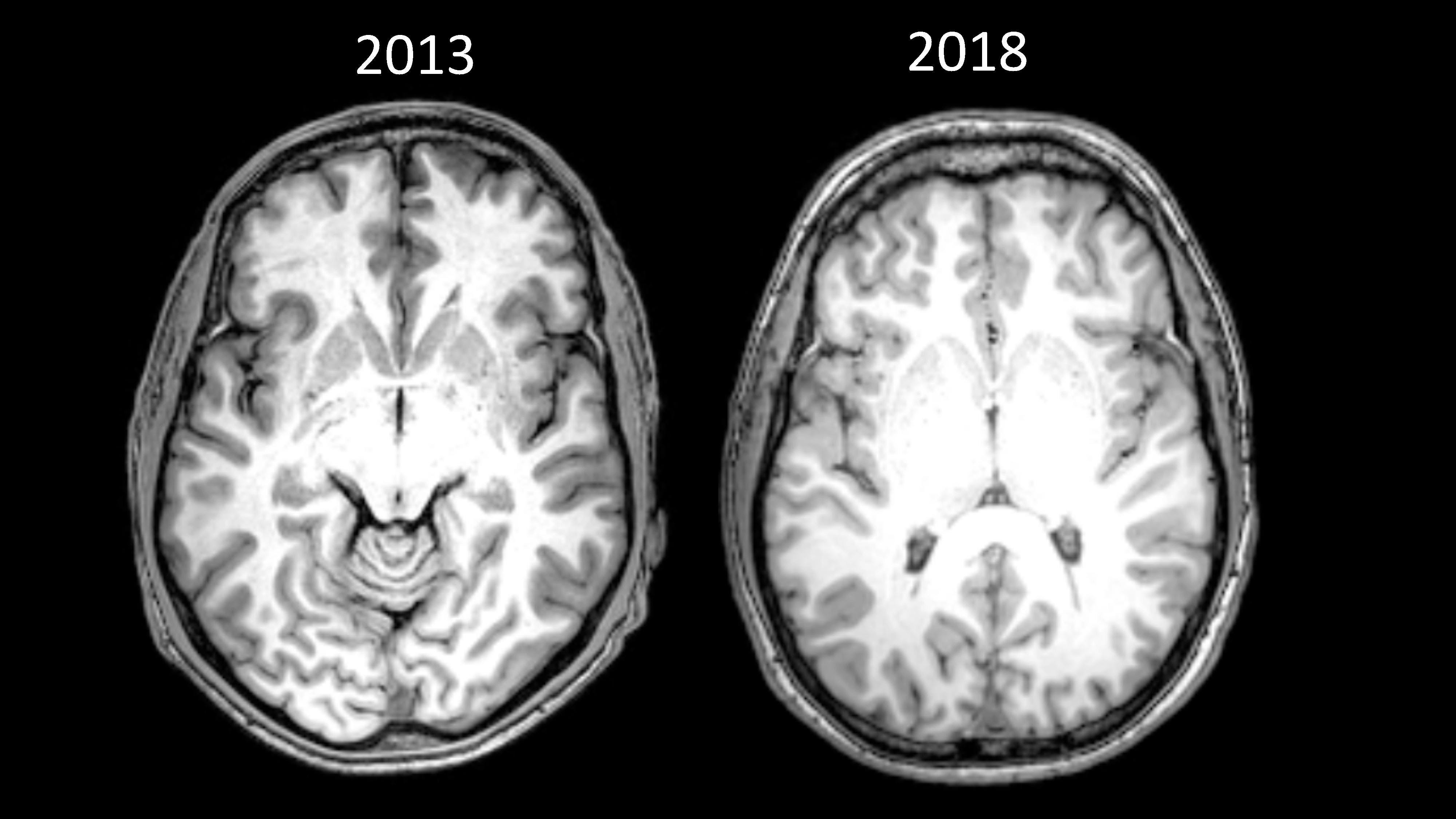
My brain was so different that the person analysing the scans could not compare the standard visual markers by eye (see the note above for a more technical explanation).
It is difficult to specifically account for what caused these changes. In the four and a half years between the scans, I radically overhauled many aspects of my life, including diet, exercise, and sleep. I also went back to college and, of course, I stopped taking heroin.
But for me, present moment awareness provided the foundations for all of these changes. From the day I was introduced to mindfulness, everything changed. It gave me a tool to cope with my greatest adversary, anxiety, and everything just flowed from there.
Emotional regulation
Research shows that a regular mindfulness practice significantly weakens the amygdala’s ability to hijack your emotions. This happens in two ways. First, the amygdala decreases in physical size. Second, connections between the amygdala and the parts of the cortex associated with fear are weakened, while connections associated with higher-order brain functions (i.e. self-awareness) are strengthened.
My own mindfulness practice has given me both of these gifts. I have literally shrunk the fear centre of my brain, and as a result, I simply don’t feel fear and anxiety like I used to. Stressful events still challenge me, but by creating a space between stimulus and response, I am no longer hijacked by my emotions.
Attention and focus
The area of the brain associated with attention is a structure called the anterior cingulate cortex. It has also been linked to self-regulation and flexible thinking — the opposite of compulsive and rigid thinking.
Research has found increased volume in this area of the brain after mindfulness practice. What’s more, when the connections between the amygdala and the rest of the cortex get weaker (i.e. the areas associated emotional hi-jacking), attentional control becomes stronger.
One study showed that practising mindfulness for only 20 minutes per day for five days can lead to improvements in attention, while a more recent study showed that a brief mindfulness intervention improves attention in complete novices.
Self-awareness
“Self” means your self-concept, your story — who you think you are. If you are suffering in some way, like I was with anxiety, disconnecting from “self” will give you the freedom to experience a greater sense of wellbeing.
Through improved self-awareness, mindfulness can provide a detachment from the self. Instead of being controlled by your self-concept, an ability to observe or experience the old you will emerge.
Although research in this area is only just emerging, some promising studies have targeted an area known as the default mode network (DMN), also known as the wandering “Monkey Mind”.
The DMN is active when our minds are directionless, aimlessly drifting from thought to thought. This has been linked to rumination and overthinking, which can be extremely counterproductive to our personal wellbeing.
Mindfulness has been found to decrease activation of the DMN, and in effect, to quieten our busy minds. In one study, regions of the DMN showed reduced activation in meditators compared to non-meditators, which has been interpreted as a diminished reference to self.
Biophoton
Jump to navigationJump to search
Biophotons (from the Greek βίος meaning “life” and φῶς meaning “light”) are photons of light in the ultraviolet and low visible light range that are produced by a biological system. They are non-thermal in origin, and the emission of biophotons is technically a type of bioluminescence, though bioluminescence is generally reserved for higher luminance luciferin/luciferase systems. The term biophoton used in this narrow sense should not be confused with the broader field of biophotonics, which studies the general interaction of light with biological systems.
Biological tissues typically produce an observed radiant emittance in the visible and ultraviolet frequencies ranging from 10−17 to 10−23 W/cm2 (approx 1-1000 photons/cm2/second).[1] This low level of light has a much weaker intensity than the visible light produced by bioluminescence, but biophotons are detectable above the background of thermal radiation that is emitted by tissues at their normal temperature.
While detection of biophotons has been reported by several groups,[2][3][4] hypotheses that such biophotons indicate the state of biological tissues and facilitate a form of cellular communication are still under investigation,[5][6] and claims that biophotons are responsible for physical healing are unsupported.[citation needed] Alexander Gurwitsch, who discovered the existence of biophotons, was awarded the Stalin Prize in 1941 for his mitogenic radiation work.[7]
Detection and measurement
Biophotons may be detected with photomultipliers or by means of an ultra low noise CCD camera to produce an image, using an exposure time of typically 15 minutes for plant materials.[8][9] Photomultiplier tubes have also been used to measure biophoton emissions from fish eggs,[10] and some applications have measured biophotons from animals and humans. [11][12][13]
The typical observed radiant emittance of biological tissues in the visible and ultraviolet frequencies ranges from 10−17 to 10−23 W/cm2 with a photon count from a few to nearly 1000 photons per cm2 in the range of 200 nm to 800 nm.[1]
Proposed physical mechanisms
Chemi-excitation via oxidative stress by reactive oxygen species and/or catalysis by enzymes (i.e., peroxidase, lipoxygenase) is a common event in the biomolecular milieu.[14] Such reactions can lead to the formation of triplet excited species, which release photons upon returning to a lower energy level in a process analogous to phosphorescence. That this process is a contributing factor to spontaneous biophoton emission has been indicated by studies demonstrating that biophoton emission can be increased by depleting assayed tissue of antioxidants[15] or by addition of carbonyl derivatizing agents.[16] Further support is provided by studies indicating that emission can be increased by addition of reactive oxygen species.[17]
Plants
Imaging of biophotons from leaves has been used as a method for Assaying R Gene Responses. These genes and their associated proteins are responsible for pathogen recognition and activation of defense signaling networks leading to the hypersensitive response,[18] which is one of the mechanisms of the resistance of plants to pathogen infection. It involves the generation of reactive oxygen species (ROS), which have crucial roles in signal transduction or as toxic agents leading to cell death.[19]
Biophoton have been observed in stressed plant’s roots, too. In healthy cells, the concentration of ROS is minimized by a system of biological antioxidants. However, heat shock and other stresses changes the equilibrium between oxidative stress and antioxidant activity, for example, the rapid rise in temperature induces biophoton emission by ROS.[20]
Theoretical biophysics
Hypothesized involvement in cellular communication
In the 1920s, the Russian embryologist Alexander Gurwitsch reported “ultraweak” photon emissions from living tissues in the UV-range of the spectrum. He named them “mitogenetic rays” because his experiments convinced him that they had a stimulating effect on cell division.[21]
Biophotons were claimed to have been employed by the Stalin regime to diagnose cancer. The method has not been tested in the West. However, failure to replicate his findings and the fact that, though cell growth can be stimulated and directed by radiation this is possible only at much higher amplitudes, evoked a general skepticism about Gurwitsch’s work. In 1953 Irving Langmuir dubbed Gurwitsch’s Mitogenetic Rays pathological science. Commercial products, therapeutic claims and services supposedly based on his work appear at present to be best regarded as such.[citation needed]
But in the later 20th century Gurwitsch’s daughter Anna, along with Colli, Quickenden and Inaba separately returned to the subject, referring to the phenomenon more neutrally as “dark luminescence”, “low level luminescence”, “ultraweak bioluminescence”, or “ultraweak chemiluminescence”.[citation needed] Their common basic hypothesis was that the phenomenon was induced from rare oxidation processes and radical reactions.
In the 1970s Fritz-Albert Popp and his research group at the University of Marburg (Germany) showed that the spectral distribution of the emission fell over a wide range of wavelengths, from 200 to 750 nm.[22] Popp proposed that the radiation might be both semi-periodic and coherent.[citation needed]
One biophoton mechanism focuses on injured cells that are under higher levels of oxidative stress, which is one source of light, and can be deemed to constitute a “distress signal” or background chemical process is yet to be demonstrated.[citation needed] The difficulty of teasing out the effects of any supposed biophotons amid the other numerous chemical interactions between cells makes it difficult to devise a testable hypothesis. A 2010 review article discusses various published theories on this kind of signaling.[23]
Pseudoscience
Many claims with no scientific proof have been made for cures and diagnosis using biophotons.[24] An appraisal of “biophoton therapy” by the IOCOB[25] notes that biophoton therapy claims to treat a wide variety of diseases, such as malaria, Lyme disease, multiple sclerosis, schizophrenia, and depression, but that all these claims remain unproven. F. Popp, a researcher who investigates biophoton emission, concludes that the complexity of cellular chemical reactions in living systems is such that it excludes the possibility to create a machine to selectively heal systems using biophotons, but there are always people who believe in these “miracles.”[25][26]
Quantum medicine
This claims:
“The quantum level possesses the highest level of coherence within the human organism. Sick individuals with weak immune systems or cancer have poor and chaotic coherence with disturbed biophoton cellular communication. Therefore, disease can be seen as the result of disturbances on the cellular level that act to distort the cell’s quantum perspective. This causes electrons to become misplaced in protein molecules and metabolic processes become derailed as a result. Once cellular metabolism is compromised the cell becomes isolated from the regulated process of natural growth control.”[27]
A review of the American Academy of Quantum Medicine concludes that many quantum medicine practitioners are not licensed as health care professionals, that quantum medicine uses scientific terminology but is nonsense, and that the practitioners have created “a nonexistent ‘energy system’ to help peddle products and procedures to their clients.”[24]
See also
Notes
- ^ Jump up to:a b Popp, Fritz (2003). “Properties of biophotons and their theoretical implications”. Indian Journal of Experimental Biology. 41 (5): 391–402. PMID 15244259.
- ^ Takeda, Motohiro; Kobayashi, Masaki; Takayama, Mariko; Suzuki, Satoshi; Ishida, Takanori; Ohnuki, Kohji; Moriya, Takuya; Ohuchi, Noriaki (2004). “Biophoton detection as a novel technique for cancer imaging”. Cancer Science. 95 (8): 656–61. doi:10.1111/j.1349-7006.2004.tb03325.x. PMID 15298728.
- ^ Rastogi, Anshu; Pospíšil, Pavel (2010). “Ultra-weak photon emission as a non-invasive tool for monitoring of oxidative processes in the epidermal cells of human skin: Comparative study on the dorsal and the palm side of the hand”. Skin Research and Technology. 16 (3): 365–70. doi:10.1111/j.1600-0846.2010.00442.x. PMID 20637006.
- ^ Niggli, Hugo J. (1993). “Artificial sunlight irradiation induces ultraweak photon emission in human skin fibroblasts”. Journal of Photochemistry and Photobiology B: Biology. 18 (2–3): 281–5. doi:10.1016/1011-1344(93)80076-L. PMID 8350193.
- ^ Bajpai, R (2009). Biophotons: a clue to unravel the mystery of “life” – Book= Bioluminescence in Focus – a collection of illuminating essays; ed Meyer-Rochow VB; Res Signpost Trivandrum. 1. pp. 357–385.
- ^ arXiv, Emerging Technology from the. “Are there optical communication channels in our brains?”. MIT Technology Review. Retrieved 9 September 2017.
- ^ Beloussov, LV; Opitz, JM; Gilbert, SF (1997). “Life of Alexander G. Gurwitsch and his relevant contribution to the theory of morphogenetic fields”. The International Journal of Developmental Biology. 41 (6): 771–7, comment 778–9. PMID 9449452.
- ^ Bennett, Mark; Mehta, Monaz; Grant, Murray (2005). “Biophoton Imaging: A Nondestructive Method for Assaying R Gene Responses”. MPMI. 18 (2): 95–102. doi:10.1094/MPMI-18-0095. PMID 15720077.
- ^ Takeda, M; Kobayashi, M; Takayama, M; et al. (August 2004). “Biophoton detection as a novel technique for cancer”. Cancer Science. 95 (8): 656–61. doi:10.1111/j.1349-7006.2004.tb03325.x. PMID 15298728.
- ^ Yirka, Bob (May 2012). “Research suggests cells communicate via biophotons”. Retrieved 26 January 2016.
- ^ Masaki, Kobayashi; Daisuke, Kikuchi; Hitoshi, Okamura (2009). “Imaging of Ultraweak Spontaneous Photon Emission from Human Body Displaying Diurnal Rhythm”. PLOS ONE. 4 (7): e6256. Bibcode:2009PLoSO…4.6256K. doi:10.1371/journal.pone.0006256. PMC 2707605. PMID 19606225.
- ^ Dotta, B.T.; et al. (April 2012). “Increased photon emission from the head while imagining light in the dark is correlated with changes in electroencephalographic power: support for Bokkon’s biophoton hypothesis”. Neuroscience Letters. 513 (2): 151–4. doi:10.1016/j.neulet.2012.02.021. PMID 22343311.
- ^ Joines, William T.; Baumann, Steve; Kruth, John G. (2012). “Electromagnetic emission from humans during focused intent”. Journal of Parapsychology. 76 (2): 275–294.
- ^ Cilento, Giuseppe; Adam, Waldemar (1995). “From free radicals to electronically excited species”. Free Radical Biology and Medicine. 19 (1): 103–14. doi:10.1016/0891-5849(95)00002-F. PMID 7635351.
- ^ Ursini, Fulvio; Barsacchi, Renata; Pelosi, Gualtiero; Benassi, Antonio (1989). “Oxidative stress in the rat heart, studies on low-level chemiluminescence”. Journal of Bioluminescence and Chemiluminescence. 4 (1): 241–4. doi:10.1002/bio.1170040134. PMID 2801215.
- ^ Kataoka, Yosky; Cui, Yilong; Yamagata, Aya; Niigaki, Minoru; Hirohata, Toru; Oishi, Noboru; Watanabe, Yasuyoshi (2001). “Activity-Dependent Neural Tissue Oxidation Emits Intrinsic Ultraweak Photons”. Biochemical and Biophysical Research Communications. 285 (4): 1007–11. doi:10.1006/bbrc.2001.5285. PMID 11467852.
- ^ Boveris, A; Cadenas, E; Reiter, R; Filipkowski, M; Nakase, Y; Chance, B (1980). “Organ chemiluminescence: Noninvasive assay for oxidative radical reactions”. Proceedings of the National Academy of Sciences. 77 (1): 347–351. Bibcode:1980PNAS…77..347B. doi:10.1073/pnas.77.1.347. PMC 348267. PMID 6928628.
- ^ Iniguez, A. Leonardo; Dong, Yuemei; Carter, Heather D; Ahmer, Brian M. M; Stone, Julie M; Triplett, Eric W (2005). “Regulation of Enteric Endophytic Bacterial Colonization by Plant Defenses”. Molecular Plant-Microbe Interactions. 18 (2): 169–78. doi:10.1094/MPMI-18-0169. PMID 15720086.
- ^ Kobayashi, M; Sasaki, K; Enomoto, M; Ehara, Y (2006). “Highly sensitive determination of transient generation of biophotons during hypersensitive response to cucumber mosaic virus in cowpea”. Journal of Experimental Botany. 58 (3): 465–72. doi:10.1093/jxb/erl215. PMID 17158510.
- ^ Kobayashi, Katsuhiro; Okabe, Hirotaka; Kawano, Shinya; Hidaka, Yoshiki; Hara, Kazuhiro (2014). “Biophoton Emission Induced by Heat Shock”. PLOS ONE. 9 (8): e105700. Bibcode:2014PLoSO…9j5700K. doi:10.1371/journal.pone.0105700. PMC 4143285. PMID 25153902.
- ^ Gurwitsch, A. A (1988). “A historical review of the problem of mitogenetic radiation”. Experientia. 44(7): 545–50. doi:10.1007/bf01953301. PMID 3294029.
- ^ Wijk, Roeland Van; Wijk, Eduard P.A. Van (2005). “An Introduction to Human Biophoton Emission”. Complementary Medicine Research. 12 (2): 77–83. doi:10.1159/000083763. PMID 15947465.
- ^ Cifra, Michal; Fields, Jeremy Z; Farhadi, Ashkan (2011). “Electromagnetic cellular interactions”. Progress in Biophysics and Molecular Biology. 105 (3): 223–46. doi:10.1016/j.pbiomolbio.2010.07.003. PMID 20674588.
- ^ Jump up to:a b Barrett, M.D., Stephen. “Some Notes on the American Academy of Quantum Medicine (AAQM)”. Quackwatch.org. Retrieved 8 May 2013.
- ^ Jump up to:a b “Biophoton therapy: an appraisal”. Archived from the original on 16 June 2013. Retrieved 8 May 2013.
- ^ “Biophotons and biontology”. 2005-12-16. Retrieved 8 May 2013.
- ^ Stephen Linsteadt, N.D, published in an ANMA newsletter
External links
- Marco Bischof’s Bibliography on biophoton research and related subjects
- G.J. Hyland’s Fundaments of Coherence in Biology
- How biophotons work (in German) by Heidi Kühnert
- Photonics TechnologyWorld, Our Bodies, Our Photons. October 1998 Edition.
- Tilbury, Gregg, Percival, Matich: “Ultraweak Chemiluminescence from Human Blood Plasma“
- F.A. Popp, et al., Recent Advances in Biophoton Research and its Application
- F.A. Popp, Biophotonics
Reference
Beloussov, L.V, V.L. Voeikov, V.S. Martynyuk. Biophotonics and Coherent Systems in Biology, Springer, 2007. ISBN 978-0387-28378-4